Pricenomics has put out a data analysis challenge as part of an effort to promote and recruit for their freelance portion of the The Priceonomics Data Studio. The challenge revolves around a fictional company called “Treefort BnB”, which has released a dataset of their treehouse listings. It seems to me like it could be pretty cool to freelance for Pricenomics as I have enjoyed reading their blog posts in the past, so I decided to solve the puzzle.
The problem and my motivation
The basic goal is to determine the median price of a booking for the the hundred most represented cities by number of listings. The technical portion of the application for the freelance gig is restricted to the specific computation mentioned above, but it seemed to me like a somewhat more extended analysis and exposition could make for a nice blog post (an opportunity not to be wasted). So in what follows I’ll show how I would solve the basis challenge using Python’s pandas library. If you haven’t seen pandas in action before this should give a good idea of how it can be useful for solving simple analysis problems. After solving the basic problem I’ll show how I would go about poking around the dataset to learn more about TreefortBnB and show off some more pandas functionality.
The basic solution
If you want to follow along using Jupyter you can find all the code here.Using IPython I downloaded the data and read it into a pandas (it is conventional to import the module as pd) dataframe with
!curl https://s3.amazonaws.com/pix-media/Data+for+TreefortBnB+Puzzle.csv > Puzzle.csv
df = pd.read_csv("./Puzzle.csv")
We can inspect the first few rows by calling head
df.head(5)
which in a Jupyter notebook will render nicely as an HTML table:
| Unique id | City | State | $ Price | # of Reviews | |
|---|---|---|---|---|---|
| 0 | 1 | Portland | OR | 75 | 5 |
| 1 | 2 | San Diego | CA | 95 | 3 |
| 2 | 3 | New York | NY | 149 | 37 |
| 3 | 4 | Los Angeles | CA | 199 | 45 |
| 4 | 5 | Denver | CO | 56 | 99 |
So we have columns corresponding to a unique id (it’s a good idea to check that it actually is unique!), a state, a city a price and total number of reviews for each listing. Having glimpsed the basic layout of the data, one can plan out a sequence of operations to convert the full table into desired summary. Here is one way to do this:
basicsummary = df.assign(City = df.City.str.title()) \
                 .groupby(["City","State"])["$ Price"] \
                 .describe().unstack().sort_values("count").tail(100)["50%"] \
                 .sort_values(ascending=False).to_frame() \
                 .rename(columns = {"50%":"median price ($)"})
basicsummary.head(5)
| median price ($) | ||
|---|---|---|
| City | State | |
| Indianapolis | IN | 650 |
| Malibu | CA | 304 |
| Park City | UT | 299 |
| Truckee | NV | 275 |
| Healdsburg | CA | 275 |
That first chunk of Python deserves a bit of explanation, which I am happy to provide.
- The first line converts all the city names to title case. This is necessary because the original column contains rows with both title and lower cases (e.g both “New York” and “new york”).
- The second line creates a grouping data structure based on the city and ctate and pulls out the price in each group (the other columns aren’t needed in this exercise). The grouping is based on both cities and states to avoid grouping distinct cities that happen to have the same name (e.g. both Carmel, California and Carmel, Indiana are present in this dataset).
- The third line is perhaps the most obscure. In it I make use of
pandasusefuldescribemethod, which returns several statistics about a column, including the total number of entries (ascount) and the median (as50%). Theunstackmethod is used to get these statistics into columns, from which point we can pull out the hundred most numerous cities and extract the median price. - The fourth line sorts the resulting “
Series” data structure by price and converts the result to a dataframe. - The last line simply renames the “50%” to “median price ($)”.
These five lines, counted as such by way of an ad-hoc continuation break up, are not necessarily the most Pythonic, but more or less reflect how I think about the steps in this exercise. I oftentimes find myself chaining method calls like this when working with pandas interactively in Jupyter or vanilla IPython, as it allows me to build up a single operation from many while getting the output by evaluating the statement in one go.
An exploratory analysis and improved solution
The above exercise focused on on median prices. This is perhaps a reasonable metric to get a sense for the typical sort of bookings one might expect to make, since it is robust to possible extreme outliers which might be present in the data. One of the nice things about using pandas interactively, however, is that we don’t have to guess, when we can see! As was already mentioned, the describe method returns a bunch of statistics which can be useful in developing a rough idea of the distribution of data in a column. We are interested in the distributions of prices in particular:
df["$ Price"].describe().to_frame() #The call to `to_frame` is a bit superfluous (I did it here to get a nice HTML table).
| $ Price | |
|---|---|
| count | 42802.000000 |
| mean | 187.117074 |
| std | 263.002109 |
| min | 10.000000 |
| 25% | 90.000000 |
| 50% | 130.000000 |
| 75% | 200.000000 |
| max | 10000.000000 |
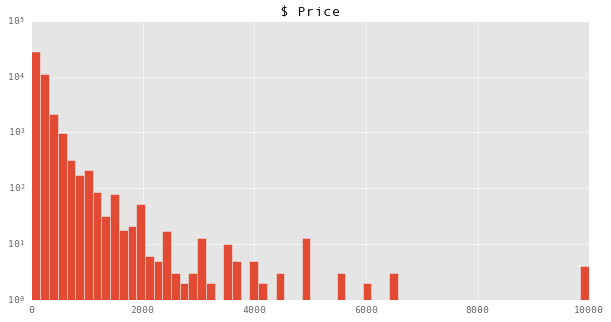
By comparing the ratio of the mean and the standard deviation, also known as the coefficient of variation, we get a sense that the distribution is somewhat dispersed to the right, as prices do not take on negative values. Furthermore we see what looks like an absurd maximum booking price of $10000. Perhaps this is Paris Hilton’s gold and sapphire plated Redwood penthouse? We can get a better idea of whats going on by looking at a graphical representation of the distribution:
df["$ Price"].hist(bins = 64,log=True)

We find that there are indeed a few listings priced at $10000 (note that the y axis is on a logarithmic scale), and that they appear to be well separated from the rest of the data. One’s imagination can run wild about the possible sorts of things this could mean about these bookings. However, it is useful to constrain one’s imagination by taking a look at the data. In pandas is it easy to select rows by criteria in the columns:
df[df["$ Price"] > 5000]
| Unique id | City | State | $ Price | # of Reviews | |
|---|---|---|---|---|---|
| 2819 | 2820 | San Francisco | CA | 10000 | 31 |
| 5135 | 5136 | San Francisco | CA | 6000 | 11 |
| 8328 | 8329 | Chicago | IL | 6500 | 1 |
| 8638 | 8639 | Indianapolis | IN | 5500 | 0 |
| 8867 | 8868 | Park City | UT | 10000 | 1 |
| 10332 | 10333 | Park City | UT | 6500 | 0 |
| 13431 | 13432 | Queens | NY | 6500 | 0 |
| 17195 | 17196 | Boston | MA | 5225 | 0 |
| 20279 | 20280 | New York | NY | 5600 | 0 |
| 23817 | 23818 | Park City | UT | 5500 | 0 |
| 26232 | 26233 | Park City | UT | 10000 | 0 |
| 28626 | 28627 | Miami Beach | FL | 10000 | 0 |
| 35136 | 35137 | Miami Beach | FL | 6000 | 0 |
| 38261 | 38262 | Miami Beach | FL | 5750 | 0 |
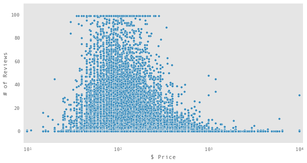
By looking at additional columns of these expensive listings we get a clue as to what might be going on. Most of these listings have no reviews. While the challenge didn’t offer any specific hints as to what one was to learn by computing median prices, the spirit of it suggest that the goal was to provide insight into a “typical” Treefort BnB experience. It stands to reason that listing without reviews have possibly never been booked, so that even though they are in the data set they may not be relevant to the larger questions we are interested in. In contrast, one would imagine that listings with many reviews are at least significant to the Treefort BnB user experience, inasmuchas users have written about them. So what does any of this have to do with prices? We can get a sense for this by doing:
df.plot(x="$ Price",y ="# of Reviews",kind='scatter',
        logx=True,xlim = [9,11000],ylim = [-10,110])

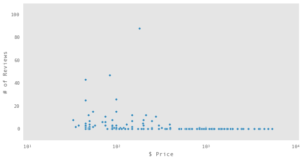
Notice how there is a clustering of points with zero or one hundred reviews? The points in the zero cluster extend significantly into the high price regime. It is hard to tell from the plots exactly how important these zero review points are to our overall problem, but they at least suggest we should look further into it. To start we can take at look at the same type of scatter plot, restricted to the bookings in Indianapolis, which which had the highest median prices in our initial analysis
df[df.City == "Indianapolis"].plot(x="$ Price",y ="# of Reviews",kind='scatter',
                                   logx=True,xlim = [9,11000],ylim = [-10,110])

Yikes! It looks like Indianapolis has a bunch of listing with no reviews, and that they probably are a big part of why it came out on top in our naive median price analysis. We can get a quantitative view of the larger picture by separating the reviewed from the unreviewed and taking a peak at some statistics:
is_reviewed = df["# of Reviews"] > 0
df.groupby(is_reviewed)["$ Price"].describe().to_frame().unstack()
| 0 | ||||||||
|---|---|---|---|---|---|---|---|---|
| count | mean | std | min | 25% | 50% | 75% | max | |
| # of Reviews | ||||||||
| False | 16000 | 238.025500 | 365.393895 | 10 | 100 | 150 | 250 | 10000 |
| True | 26802 | 156.726252 | 168.202838 | 10 | 85 | 125 | 185 | 10000 |
We see that about 40% of the total listings are unreviewed with their prices shifted to the right (both in terms of mean and median). Furthermore there are some rather suspicious looking quantiles for these unreviewed listings ($100, $150, $250… what are the odds?!). All of this seems to add credibility to the initial idea that filtering out listings that haven’t been reviewed might give a better picture of what to expect when booking.
With this in mind I set out for a better version of the basic result above. I also thought it could be useful to group location with the same median price into the same row with a slightly different formatting, which could then be indexed by a price rank. This lead me to the following lines of code:
refinedsummary = df.get(df["# of Reviews"] > 0) \
                   .assign(Location = df.City.str.title()+df.State.apply(lambda s: ' ('+s+')')) \
                   .groupby("Location")["$ Price"].describe().unstack() \
                   .sort_values("count").tail(100) \
                   .reset_index().groupby("50%")["Location"].apply(lambda x: "%s" % ' / '.join(x)) \
                   .sort_index(ascending=False).to_frame() \
                   .reset_index().rename(columns = {"50%":"median price ($)"})
refinedsummary.set_index(refinedsummary.index+1,inplace = True)
refinedsummary.index.rename("rank",inplace = True)
refinedsummary.head(15)
| median price ($) | Location | |
|---|---|---|
| rank | ||
| 1 | 300.0 | Carmel (CA) |
| 2 | 225.0 | Healdsburg (CA) / Malibu (CA) |
| 3 | 200.0 | Incline Village (NV) / Laguna Beach (CA) / Truckee (NV) |
| 4 | 199.0 | Hermosa Beach (CA) |
| 5 | 184.5 | Napa (CA) |
| 6 | 179.0 | Park City (UT) |
| 7 | 177.5 | Sunny Isles Beach (FL) |
| 8 | 175.0 | Sonoma (CA) |
| 9 | 165.0 | New York (NY) |
| 10 | 162.0 | Manhattan Beach (CA) |
| 11 | 157.5 | La Jolla (CA) |
| 12 | 150.0 | Sausalito (CA) / Beverly Hills (CA) / Newport Beach (CA) / Venice (CA) / Boston (MA) / Austin (TX) / San Francisco (CA) |
| 13 | 149.0 | Marina Del Rey (CA) |
| 14 | 148.0 | Mill Valley (CA) |
| 15 | 130.0 | Santa Monica (CA) / Miami Beach (FL) |
With this we see that Indianapolis has been pushed out of the top ranks, which are now occupied by somewhat more sensible places for expensive treehouses (to the extent that such a thing exists).
There are of course, other aspects of the data we might want to consider. For example, where should you head if you want the widest selection of treeforts? By, now, you may have an idea of how I would go about answering this question…
nlistings = df.get(df["# of Reviews"] > 0) \
         .groupby(["City","State"]).count()["$ Price"] \
         .sort_values(ascending = False).to_frame() \
         .rename(columns = {"$ Price":"total listings"})
nlistings.head(10)
| total listings | ||
|---|---|---|
| City | State | |
| New York | NY | 5597 |
| Brooklyn | NY | 3017 |
| San Francisco | CA | 2455 |
| Los Angeles | CA | 1941 |
| Austin | TX | 1495 |
| Chicago | IL | 875 |
| Washington | DC | 836 |
| Miami Beach | FL | 790 |
| Portland | OR | 586 |
| Seattle | WA | 573 |
At first glance (say, for the first ten seconds) this looks reasonable, although there is a question of whether or not or exactly how Brooklyn is not contained in New York. But let’s assume that “New York” means every borough except Brooklyn. The data show that there are 3017 reviewed listings in Brooklyn. Are there over three thousand treehouses in Brooklyn? Granted, there are quite a few trees. But treehouses are sufficiently rare that you might make it into the New York Times for building one there. Still, exactly how many is not obvious but…
WARNING!!! YOU ARE ENTERING THE FERMI ESTIMATION ZONE. HOLD ON TO YOUR POWERS OF TWO AND TEN!
… to get things started lets say that there are about as many trees as there are people. So, a couple million. Now, one expects that a great deal, say 90%, of these tree are going to be found in public parks where one is likely to have a hard time constructing a treefort, not to say anything about renting it out. We still have hundreds of thousands of trees to work with though. Now imagine you are walking on a street in Brooklyn and spot a bunch of trees (if you hare having a hard time imagining use Google Street View). Most of the trees that you see are sort of lining the streets and sidewalks, which also would make for construction difficulties. Let’s be generous though and say that 10% of the remaining trees can be found in backyards and other places suitable for treehouse construction. There are ten thousand-ish trees (from tiny saplings to grand oaks) left to work with. And yet, the above table states that there several thousand listings in the same area. Are we to believe that every third tree in Brooklyn has a treehouse on it and all of them are for lease through Treefort BnB!?
Of course we don’t, because we know that the data are fake and Treefort BnB does not exist. But I wanted to end with that little Fermi estimation paragraph because it shows how data of this sort usually raises many interesting questions, including those about the accuracy of the data itself, which is something that freelancers should definitely keep in mind when working with a client’s data.